how many galaxies?
- Mar 20, 2024
- 14 min read
Updated: Mar 7, 2025
by Kevin C. Moore and Sohei Yasuda
A colleague, Dr. Pat Thompson, recently posed the following question:
The James Webb Telescope Deep Field photograph has a field of view of 2.4 arc minutes (2.4/60 degrees) in height and width (5.76 square arc minutes). NASA counted approximately 45,000 galaxies in it.

The question is, if this is a representative sample of the entire sky, how many galaxies are in the visible universe? (By the way, one of the primary cosmological assumptions is that the universe looks the same regardless of one’s position in it, so it is reasonable to assume this is a representative sample.)
This question generated a lively conversation, both within its email chain as well as within our interactions here at UGA. The gist of these conversations: quantification is a big deal!
Quantification
Eventually there will be a study guide on quantification that outlines Thompson's (2011) nuanced exposition. But for now, it is sufficient to think of quantification as understanding the quantity and its amount conveyed by a measure. For instance, if we say Kevin's height is 6.0 feet, you might understand that as a measure of the span from the bottom of Kevin's feet to the top of his head using a straight segment that is defined as 1-foot long, with 6 iterations of those end-to-end covering that span. Although this description may seem cumbersome, such an unpacking is critical to answering the above question. That is, it requires answering what is meant by a field of view of “2.4 arc minutes (2.4/60 degrees) in height and width (5.76 square arc minutes)”?
For ease of illustration and discussion, we will use a stated field of view of π/6 radians in height and width, which we might call a field of view of π/6*π/6 square radians. As shown below, we can privilege either the dimensions aspect of this statement or the area aspect of this statement. Furthermore, we will see that a field of view of π/6 radians in height and width does not necessarily mean a field of view of π/6*π/6 square radians in terms of covered universe. This stems from how field of view is quantified and how that relates to determining the image region captured.
Assumption
An assumption is that the reception of light can be modeled as a linear projection from the source to the receiver as in Figure 1. Consistent with Figure 6, this assumption yields a field of view that scales proportionally with distance from the receiver. We will explore different fields of view forms, but all will entail a field of view with dimensions that scale proportionally. The assumption of light as a linear projection is important because it enables reducing an image to the surface of a sphere (a three-dimensional projection onto a two-dimensional surface). A technique that captures an entire sphere also captures the entire (visible) universe, as all light sources can be projected onto that sphere with the assumption in Figure 1.

Figure 1. A light source (right) and a receiver (left), with the captured field scaling proportionally.
Interpretation 1
For interpretation 1, we present three different cases. We group these interpretations together because within each case, a stated field of view corresponds to the same two-dimensional shape, three-dimensional shape, linear surface area of each, and angular surface area of each no matter the region of space we are pointing the camera (or cropping the image). As seen in the second interpretation, this need not be the case.
Interpretation 1a. In the first case, we consider the field of view to be defined by great circles. The stated dimensions convey an angle of rotation along great circles on a sphere (a square field of view). Importantly, the great circles rotations occur along are with respect to the center of the field of view. Figure 1 is defined by such a field of view, as is Figure 2. At any layer in the two-dimensional right square pyramid or its extension, the edges of the field of view on the sphere’s surface are π/6 radii in length and lie on great circles (i.e., π/6 sphere-radii). The intersecting points of the great circles form the corners of a two-dimensional square[1]; the field of view is formed by a square projected into space such that its sides vary proportionally with respect to its distance into space.[2] The dimensions of this two-dimensional square is less than π/6 sphere-radii by π/6 radii, and is in fact 2sin(π/12), or 0.5176, sphere-radii by 0.5176 sphere-radii. Its area is approximately 0.2679492 square sphere-radii.

Figure 2. A single wedge for a great circle field of view and two examples with a sphere.
Given a spherical rectangular region defined by great circle dimensions of l and w on a sphere with radius r, the enclosed area is

Setting the radius as our unit, we have a square pyramid that defines a spherical square surface of approximately 0.287434 square radii. Because the surface of any sphere is 4π square radii, it takes approximately 43.71909 photos at our example field of view to capture the entire universe.
Interpretation 1b. For Interpretation 1b, a stated field of view defines the dimensions of the image that captures a spherical cap. In our specific example, the field of view encompasses a pitch and yaw of π/12 radians from all initial roll amounts, with a roll maintaining our center of field of view.[3] This creates a spherical cap as illustrated in Figure 3, whose projection is a cone. At any layer in the cone or its extension, the surface captured by the image is a spherical circle such that any length passing from boundary to boundary through its center is π/6 radii long. Like Interpretation 1a, π/6 refers to both angular sweep from the point of view of the camera, as well as a length along a sphere’s surface. Their values are in agreement in terms of radians and radii because distance occurs along great circles, thus maintaining a direction of rotation frames of reference from the center of the field of view. Also, like the boundary intersections in Interpretation 1a, a two-dimensional cross-section is formed. In this case, the field of view is formed by a circle projected into space such that its radius varies proportionally as its distance into space increases. The diameter of this two-dimensional circle is less than π/6 sphere-radii, and is in fact 2sin(π/12), or approximately 0.5176, sphere-radii. Its area is approximately 0.2104468 square sphere-radii.
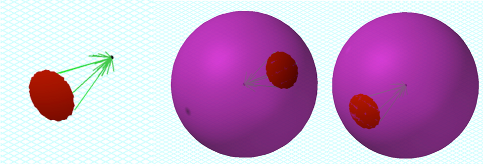
Figure 3. Spherical cap images created by a pitch of π/12 radians for any roll amount around a fixed center of view.
We know the area of a spherical cap is

with 𝜃 representing the angle pitched from the center of view. Setting the radius as our unit, we have a spherical image area of approximately 0.21409 square sphere-radii. It would take approximately 58.695 photos at that field of view to capture the entire universe. Like the previous interpretation, a uniform tiling of a sphere is impossible with this field of view.
Interpretation 1c. For Interpretation 1a, our spherical square is a quadrilateral having equal, non-parallel sides such that all interior angles are equal in magnitude. The resulting area is not π/6*π/6 square sphere-radii for the spherical surface area nor the two-dimensional square area. Similarly, our image in Interpretation 1b is not π/6*π/6 square sphere-radii, nor is it π*(π/12)^2 square sphere-radii, whether speaking about the spherical cap or its two-dimensional circle area. We are conveying the size of an image–a two-dimensional object–using quantities from the three-dimensional world it captures, and thus any calculation of area considers that three-dimensional world. It is possible to determine the area of the projected two-dimensional object, as we have above.
For Interpretation 1c, we consider the field of view to be defined strictly by area and the photo thus captures a field of view that yields the stated area on the surface of a sphere. This field of view could be of any shape, including a spherical square like that in Interpretation 1a or a spherical circle like that 1b. It could also be a spherical rectangle or other shapes as dictated by the camera. For our specific example, we can consider a field of view shape, no matter where pointing, to capture a spherical surface area of π/6*π/6 square sphere-radii, or approximately 0.274156 square sphere-radii. It would take approximately 45.83662 photos at that field of view to capture the entire universe. In this case, it is possible for a field of view to achieve uniform tiling depending on the particular shape and size (e.g., a “triangular” camera).
For our specific example, we note an alternative interpretation of the stated π/6 by π/6 square radii defines a two-dimensional view that is a π/6 square sphere-radii by π/6 square sphere-radii square. Here, the sphere-radius is defined by the radius of the sphere that intersects the four vertexes of the square and, hence, the associated spherical square. In this case, the field of view on the sphere is defined by lengths of 2arcsin(π/12) sphere-radii along great circles, or approximately 0.5297722 sphere-radii. This results in an approximate spherical surface area of 0.2945949 square sphere-radii. It would take approximately 42.65644 photos at that field of view to capture the entire universe. In this case, a uniform tiling is possible depending on the particular shape and size. This case is also equivalent in its structure to Interpretation 1a, but uses the stated area as a measure of the two-dimensional surface area rather than three-dimensional surface area.
Interpretation 2
With Interpretation 1, a stated field of view corresponds to the same shape and spherical surface area as measured using a distance unit no matter the direction in space the image is taken or from. With Interpretation 2, as we illustrate in this section, a stated field of view in both shape and surface area is dependent on where in the sky one is pointing their camera. As an alternative way to think about Interpretation 2, imagine you have the entire universe catalogued and desire to break its entirety into a systematized group of smaller photos, possibly for display purposes on a specific shell. One way to do this would be to map the surrounding universe using a coordination system. Fortunately, we can treat our catalogue as a three-dimensional projection onto a two-dimensional surface—a sphere—and such a coordinate system already exists for the sphere. This is known as a geographic coordinate system.[4]
For illustrative purposes, rather than using a longitude and latitude based on 1-degree increments, we return to our π/6 radian increments for both longitude and latitude. Figure 4 illustrates image regions based on such a system for longitude 0 ≤ λ ≤ π/2 and latitude 0 ≤ ϕ ≤ π/2. Each image region defines a field of view such that it is π/6 radians by π/6 radians with respect to longitude and latitude. This is not equivalent to saying each image region defines a field of view that is π/6 radii by π/6 radii with respect to the sphere (i.e., sphere-radii), or a field of view that is π/6 radians by π/6 radians with respect to camera yaws or pitches. A longitude coordinate is defined by a great circle. Thus, a change in latitude occurs along a great circle and corresponds to as sphere-radii measures. On the other hand, a latitude coordinate corresponds to a “horizontal” circle, with only one of those being a great circle (ϕ = 0). Hence, changes in longitude occur along a “horizontal” circle and are defined by the radius of the circle that is formed by the latitude line (e.g., lat-radii). Thus, the arc length that defines a specific change in longitude varies as one varies their latitude position. As one increases or decreases in ϕ value from 0, the boundaries for an image region decrease in the longitude rotation direction and thus define a smaller field of view with respect to square sphere-radii. This is most noticeable when comparing the first and third sets of image regions including their projections in Figure 4. In the third set, one boundary collapses to a point, or a sphere-radii measure of 0.[5]

Figure 4. A geographic coordinate system for locating photos based on π/6 increments.
In our specific case, each image region is a boundary of π/6 by π/6 by π/6 by π/6 radians. Two of those values are in sphere-radii and refer to the same length, and two of them refer to lat-radii and thus differ in lengths from each of the other 3. The area is not π/6*π/6 square radians (nor sphere-radii). Each image region is π/6*π/6 sphere-radii X lat-radii, or approximately 0.274156 sphere-radii X lat-radii. We need a total 72 image regions to display the entire universe. As we illustrate in Solutions, we can use this to estimate the number of total galaxies in the universe.
We note that one way to visualize regions of the same sphere-radii X lat-radii is provided in Figure 4. We use Figure 5 as an alternative way of visualizing such regions. Figure 5 is based on the same field of view center, but with varying latitude and longitude dimensions in order to maintain an area of 1 sphere-radii X lat-radii. In other words, the field of view maintains the same center and is always a sphere-radii by b lat-radii so that ab = 1.
Figure 5. A field of view with a fixed center, varying dimensions, but such that the area is always 1 sphere-radii X lat-radii (e.g., a sphere-radii by b lat-radii so that ab = 1). The graph indicates the spherical surface area by the y-coordinate of the point.
Solutions
Interpretation 1a Solution. Recall that the original image was stated as 2.4 arc minutes (2.4/60 degrees) in height and width (we ignore the 5.76 square arc minutes statement because Interpretation 1a uses dimensions), with approximately 45,000 galaxies in it. The image is 2.4/60 sphere-degrees by 2.4/60 sphere-degrees, or (2.4/60)*(π/180) sphere-radii by (2.4/60)*(π/180) sphere-radii. Using the area formula from above, the captured surface area is approximately 4.87387911 × 10e-7 square sphere-radii. The surface area of a sphere is 4π square sphere-radii, resulting in approximately 25783098 photos of this size to capture the entire sphere and, thus, universe. There are approximately 1.1602394 × 10e12 galaxies by this method.
Interpretation 1b Solution. As with Interpretation 1a, the image is (2.4/60)*(π/180) sphere-radii by (2.4/60)*(π/180) sphere-radii, but it forms a spherical cap rather than a spherical square. Using the area formula from above, the captured surface area is approximately 3.82793535 × 10e-7 square sphere-radii. The surface area of a sphere is 4π square sphere-radii, resulting in approximately 32828064 photos of this size to capture the entire sphere and, thus, universe. There are approximately 1.47726287 × 10e12 galaxies by this method.
Interpretation 1c Solution. Recall that the original image was stated as 5.76 square sphere-arc minutes (we ignore the 2.4 arc minutes in height and width statement because Interpretation 1c uses area), with approximately 45,000 galaxies in it. The image is 5.76/(60^2) square sphere-degrees, or 5.76/(60^2) *(π/180)^2 square sphere-radii (approximately 4.87387872 × 10e-7 square sphere-radii). The surface area of a sphere is 4π square sphere-radii, resulting in approximately 25783100 photos of this size to capture the entire sphere and, thus, universe. There are approximately 1.1602395 × 10e12 galaxies by this method.
The above solution uses the stated amount as the area on the sphere. If the stated amount is in reference to the two-dimensional square field of view, this corresponds to a spherical surface area of approximately 4.87387931× 10e-7 square sphere-radii. We would need approximately 25783098 photos of this size to capture the entire sphere and, thus, universe. There are approximately 1.1602394 × 10e12 galaxies by this method.
Interpretation 2 Solution. For Interpretation 2’s solution, we return to the stated dimensions of 2.4 arc minutes in height and width, or 2.4π/10800 radians in height and width. We could phrase this as 2.4π/10800 sphere-radii by 2.4π/10800 lat-radii. We also know that the area of a region bounded by longitudes and latitudes is

For our solution, consider the case in which a region boundary lies along the latitude defining the “equator” (ϕ = 0) and the case in which a region boundary is the pole (ϕ = π/2). Regardless, our difference in λ is 2.4π/10800 lat-radii. For the first case, ϕ varies from 0 to 2.4π/10800 sphere-radii. For the second case, ϕ varies from (π/2 - 2.4π/10800) to π/2 sphere-radii. In the first case, by the formula above our area is approximately 4.87387832 × 10e-7 square sphere-radii. In the second case, by the formula above our area is approximately 1.7013 × 10e-10 square sphere-radii. To extrapolate each case to the entire sphere and, thus, universe, we determine the density of galaxies in each respective region. Recall that the given picture is stated to have 45,000 galaxies captured. The first case yields a density of approximately 92328936094 galaxies per square sphere-radii. The second case yields a density of approximately 2.6450291 × 10e14 galaxies per square sphere-radii. A sphere has a surface area of 4π square sphere-radii. The first case yields approximately 1.1602396 × 10e12 total galaxies, while the second case yields approximately 3.3238416 × 10e15 total galaxies.
A third case is to use a region that straddles the “equator”, or ϕ varying from -1.2π/10800 sphere-radii to 1.2π/10800 sphere-radii. This results in a total number of galaxies of 1.1602396 × 10e12 galaxies. Expanding to more digits, we have 1.16023955870 × 10e12 total galaxies as compared to 1.16023962939 × 10e12 total galaxies in the first case. This subtle difference is that the first case results in a higher density of galaxies to apply to the sphere due to the smaller image region.
Summary of Solutions
Interpretation | Information | Total Number of Galaxies |
1a | Field of View Defined by Great Circles | 1.1602394 × 10e12 |
1b | Field of View Defined by a Circle | 1.4772629 × 10e12 |
1c | Field of View Defined by Stated Sphere Surface Area | 1.1602395 × 10e12 |
1c | Field of View Defined by Stated Square Surface Area | 1.1602394 × 10e12 |
2 | Field of View Defined by Geographic Coordinate System – Equator Boundary | 1.1602396 × 10e12 |
2 | Field of View Defined by Geographic Coordinate System – Pole Boundary | 3.3238416 × 10e15 |
2 | Field of View Defined by Geographic Coordinate System – Straddle Equator | 1.1602396 × 10e12 |
Interpretation 1a, 1b, 1c, Interpretation 2 Equator Boundary, and Interpretation 2 Straddle Equator each result in a similar total number of galaxies, which is to be expected due to their structures combined with the region that defines the galaxy density in Interpretation 2. Interpretation 1b is larger due to its relatively smaller area. Interpretation 2 Pole Boundary results in a noticeably greater total number of galaxies due to the relatively smaller image region as compared to the other solutions.
Other Information and Comments
Interpretation 2 is sensible if you have the entire universe photographed and you want to pull a still or define things by regions. Whereas Interpretation 1 does not always allow for one to partition an entire sphere into non-overlapping images, Interpretation 2 does. But, to generalize from a single photo to the entire universe requires using where the picture is cropped from to determine either the relative region size or its galaxy density. Interpretation 1 is sensible if wanting to convey size that is invariant across camera direction or image location, thus allowing one to generalize from the image without knowing the direction of the image (e.g., where it is cropped from). Interpretation 1 also results in the same distortion characteristics for all images if displayed at the same linear size, whereas Interpretation 2 requires different distortion characteristics if desiring to display all images at the same linear size.
Given that the phrasing of the image is with respect to the camera field of view as opposed to image field of view, with the latter requiring additional location information to determine absolute size, we presume Interpretation 1 is the most viable. Interpretation 1a is also consistent with how a camera’s angle of view is typically conveyed, or when a camera’s field of view is given in terms of angular components.

Figure 6. A standard field of view and angle of view representation, with the angle of view forming a rectangular field of view. A field of view quantified with linear units must be paired with a distance at which the field of view occurs. Alternatively, a field of view can be stated in terms of its angle of view, which is of the same dimensional values across all distances.
[1] For the purpose of this write-up, we refer to a sphere as a three-dimensional object to indicate its additional quantitative dimensions as opposed to the two-dimensional field of view.
[2] The image boundary on the sphere can also be formed from the center of the field of view by yaws of +-π/12 that follow pitches of +-π/12 combined with pitches of +-π/12 that follow yaws of +-π/12.
[3] We use these in terms of standard rotation dimensions referenced in aviation and space.
[4] A key difference exists between the quantities constituting Interpretation 1 and those of the geographic coordinate system in Interpretation 2. In the former, frames of reference are always with respect to the center of the field of view, and thus re-established with each picture so that the size of the field of view never changes. In the latter, fixed frames of reference are established using positions on a sphere and all positions and movements are then with respect to the resulting fixed system. These differences are similar to how a pilot balances frames of reference that are with respect to the plane with frames of reference defined by coordinate systems fixed independent of the plane’s position and orientation. To a pilot, pitch, yaw, and roll movements caused by the yoke are always with respect to the current heading and plane’s orientation (e.g., center of the field of view). Planetarium viewer applications can define movement in either way, depending on desire.
[5] Another way to think about this is sitting in the camera seat, placing your center of view on a boundary, and attempting to move your chair via a joystick so that you trace the boundary while always being oriented perpendicular to the boundary. If it operates as an airplane does, in Interpretation 2, you need to combine a roll with a yaw to trace a latitude. In Interpretation 1a, you can trace a boundary with only yaw or pitch movements. As noted in the previous footnote, software applications can constrain the yoke (or keypad) movements to trace geographic coordinate systems.